AESA Phased Array Beamforming: From Theory to FPGA Implementation
A simulation-driven deep dive into phased array antenna beamforming — array factor physics, electronic beam steering, sidelobe control, and grating lobe avoidance for modern AESA radar systems.
Apexia Engineering
Apexia
Active Electronically Scanned Arrays (AESAs) have become the dominant antenna architecture in modern radar, electronic warfare, and communications systems. Unlike mechanically steered dishes, an AESA steers its beam electronically — in microseconds — by adjusting the phase of each element in the array. No moving parts, no inertia, no wear.
This post walks through the core physics of phased array beamforming using real simulations generated with NumPy and SciPy. Every figure below comes from actual array factor computations, not hand-drawn approximations. We will cover how element count shapes beamwidth, how phase progression steers the beam, how amplitude tapering suppresses sidelobes, and why element spacing above half a wavelength creates dangerous grating lobes.
Why This Matters for FPGA Engineers
Beamforming is fundamentally a real-time signal processing problem. Each element needs independent phase and amplitude control updated at the pulse repetition interval. For a 256-element array at 10 kHz PRF, that is 2.56 million weight updates per second — exactly the kind of deterministic, parallel workload that FPGAs excel at.
The Array Factor: How Element Count Shapes the Beam
The array factor (AF) describes the radiation pattern produced purely by the spatial arrangement of elements, independent of the individual element pattern. For a Uniform Linear Array (ULA) with N elements spaced at distance d, the array factor at observation angle θ is the coherent sum of phasors across all elements:
Array Factor Equation
AF(θ) = Σ wₙ · exp(j·n·ψ), where ψ = 2π(d/λ)(sin θ − sin θ₀), wₙ are the element weights, and θ₀ is the steering angle. For uniform weighting (wₙ = 1/N), this simplifies to the familiar sinc-like pattern.
The critical insight: more elements means a narrower main beam. The 3 dB beamwidth of a ULA scales approximately as λ/(N·d·cos θ₀). Doubling the element count halves the beamwidth, doubling angular resolution. The simulation below shows this relationship clearly — the N=64 beam is dramatically sharper than N=8, with proportionally lower sidelobes relative to the main beam.
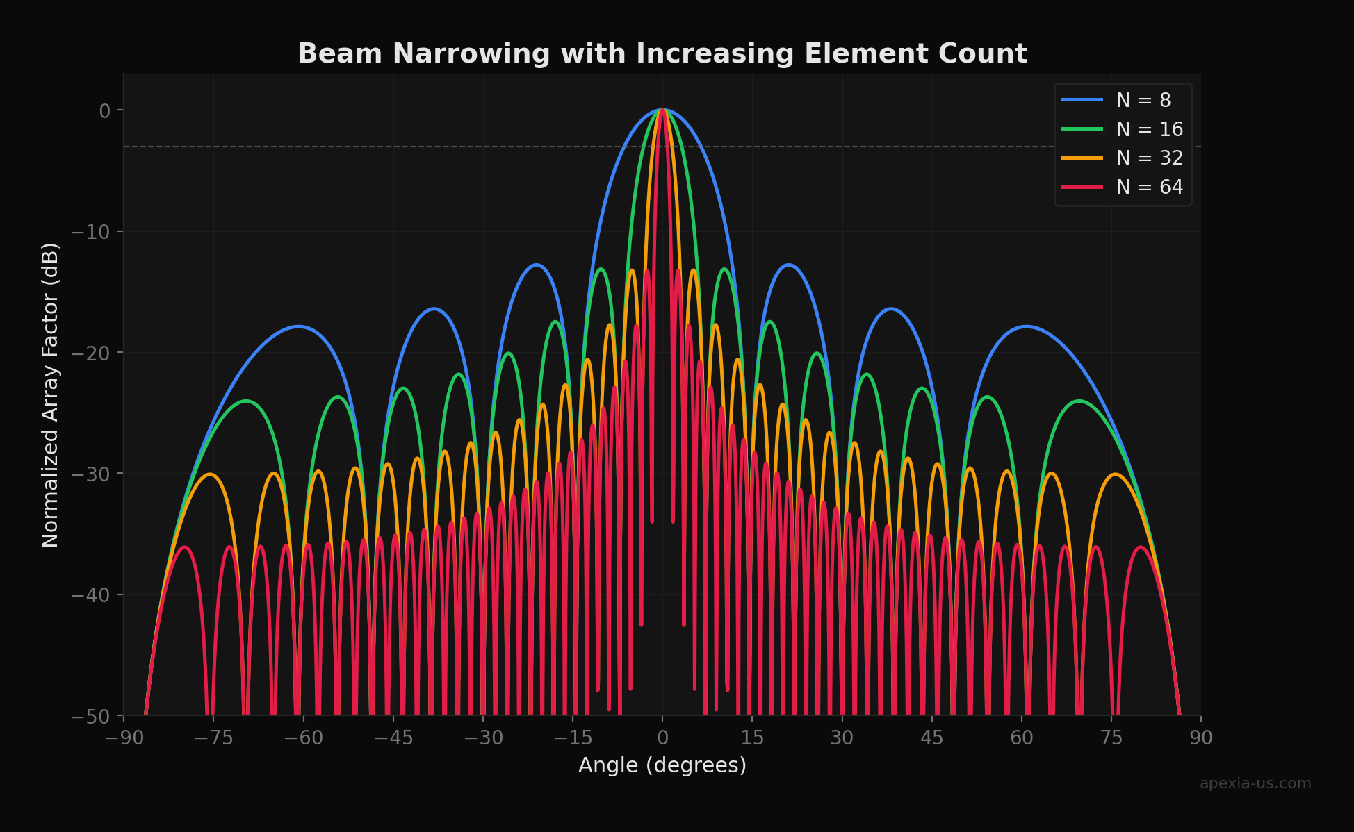
Try the interactive version below — toggle element counts on and off to see exactly how each doubling sharpens the beam and pushes the first sidelobe further down.
Electronic Beam Steering: Phase Progression Across Elements
The defining advantage of a phased array is inertialess beam steering. By applying a linear phase gradient across the elements, the main beam shifts to a new angle without any physical movement. The required phase shift for element n to steer to angle θ₀ is simply Δφₙ = 2π·n·(d/λ)·sin(θ₀).
The simulation below shows a 32-element ULA steered to 0°, 15°, 30°, and 45°. Notice how the beam broadens at larger scan angles — this is beam broadening, an inherent physical effect where the effective aperture projected onto the scan direction shrinks as cos(θ₀). At 45°, the beam is roughly 41% wider than at boresight.
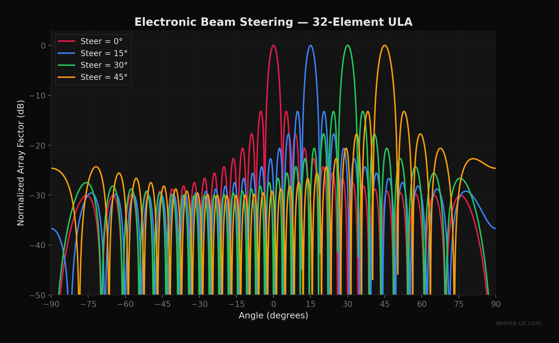
Drag the slider in the interactive version to continuously steer the beam and watch how the pattern deforms at extreme scan angles.
32-element ULA at d = λ/2 — drag the slider to steer the beam electronically
FPGA Implementation Note
In hardware, the phase shifts are typically implemented as complex weight multiplications in the digital beamformer. Each element's I/Q data is multiplied by exp(jΔφₙ) and the products are summed. On an RFSoC, this maps naturally to the DSP48E2 slices — a single 27×18 complex multiply per element, fully pipelined at the ADC sample rate.
Sidelobe Control: Amplitude Tapering for Clutter Rejection
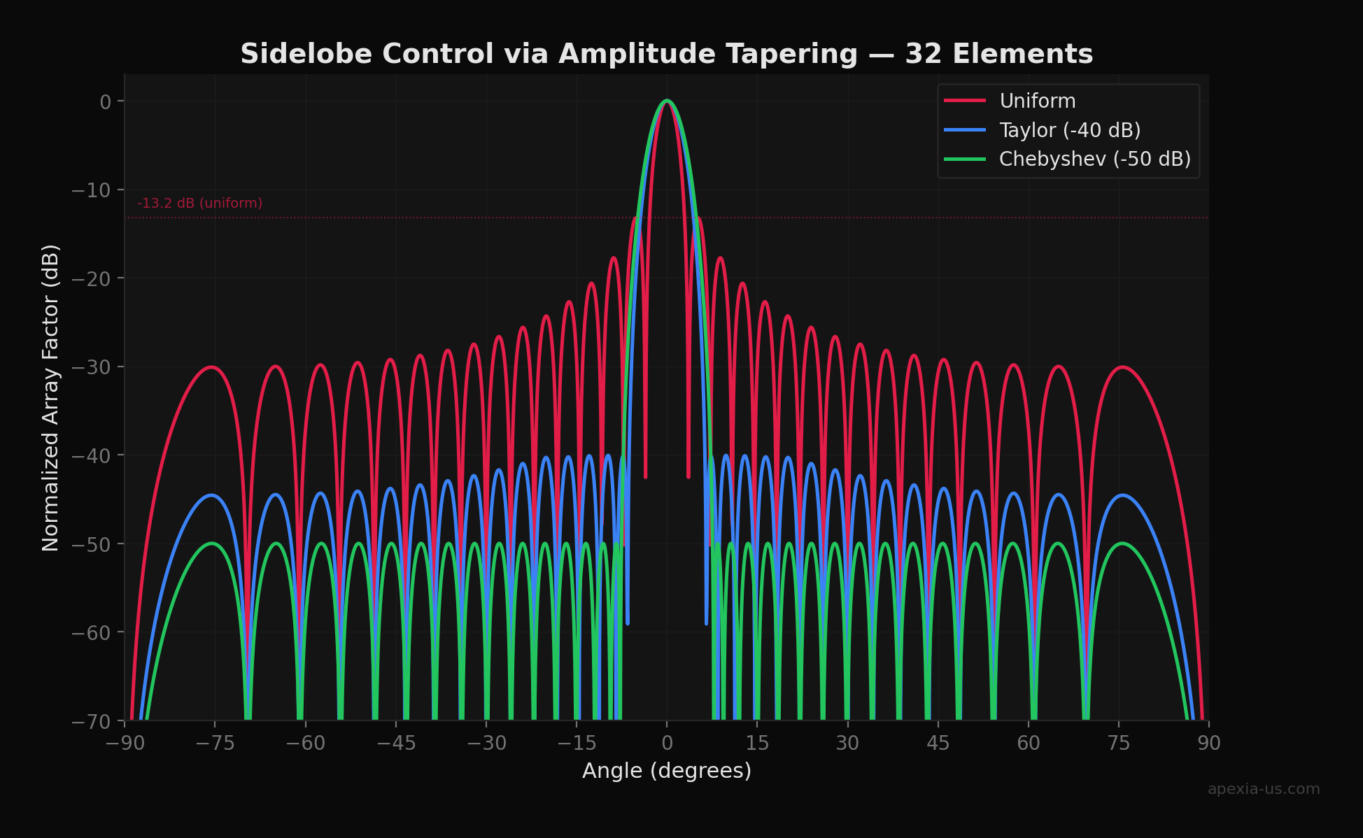
Sidelobes are the enemy of radar performance. A target return arriving through a sidelobe is indistinguishable from a weaker target in the main beam. For a uniformly weighted array, the first sidelobe sits at -13.2 dB relative to the main beam — often unacceptable for search radars operating in heavy clutter.
The solution is amplitude tapering (also called amplitude weighting or windowing). By reducing the amplitude of the outer elements relative to the center, sidelobes are suppressed at the cost of slightly broader main beams. The two most common tapers in radar are Taylor and Chebyshev:
- Taylor taper — designed for a specified sidelobe level (e.g., -40 dB) with near-constant sidelobes near the main beam, transitioning to the specified level. The nbar parameter controls how many sidelobes near the main beam are kept constant. Widely used in radar.
- Chebyshev (Dolph-Chebyshev) taper — achieves the narrowest possible main beam for a given sidelobe level. All sidelobes are at exactly the specified level. Optimal in the minimax sense but can be harder to implement with finite-precision weights.
- Uniform (no taper) — narrowest beam but -13.2 dB first sidelobe. Acceptable when clutter is not a concern or when maximum angular resolution is paramount.
| Taper | First Sidelobe | Beamwidth | Best For |
|---|---|---|---|
| Uniform | -13.2 dB | Narrowest | Maximum resolution, low clutter |
| Taylor (-40 dB, nbar=5) | -40 dB | ~15% wider | Search radar, moderate clutter |
| Chebyshev (-50 dB) | -50 dB | ~20% wider | High-clutter environments |
Grating Lobes: The Half-Wavelength Spacing Rule
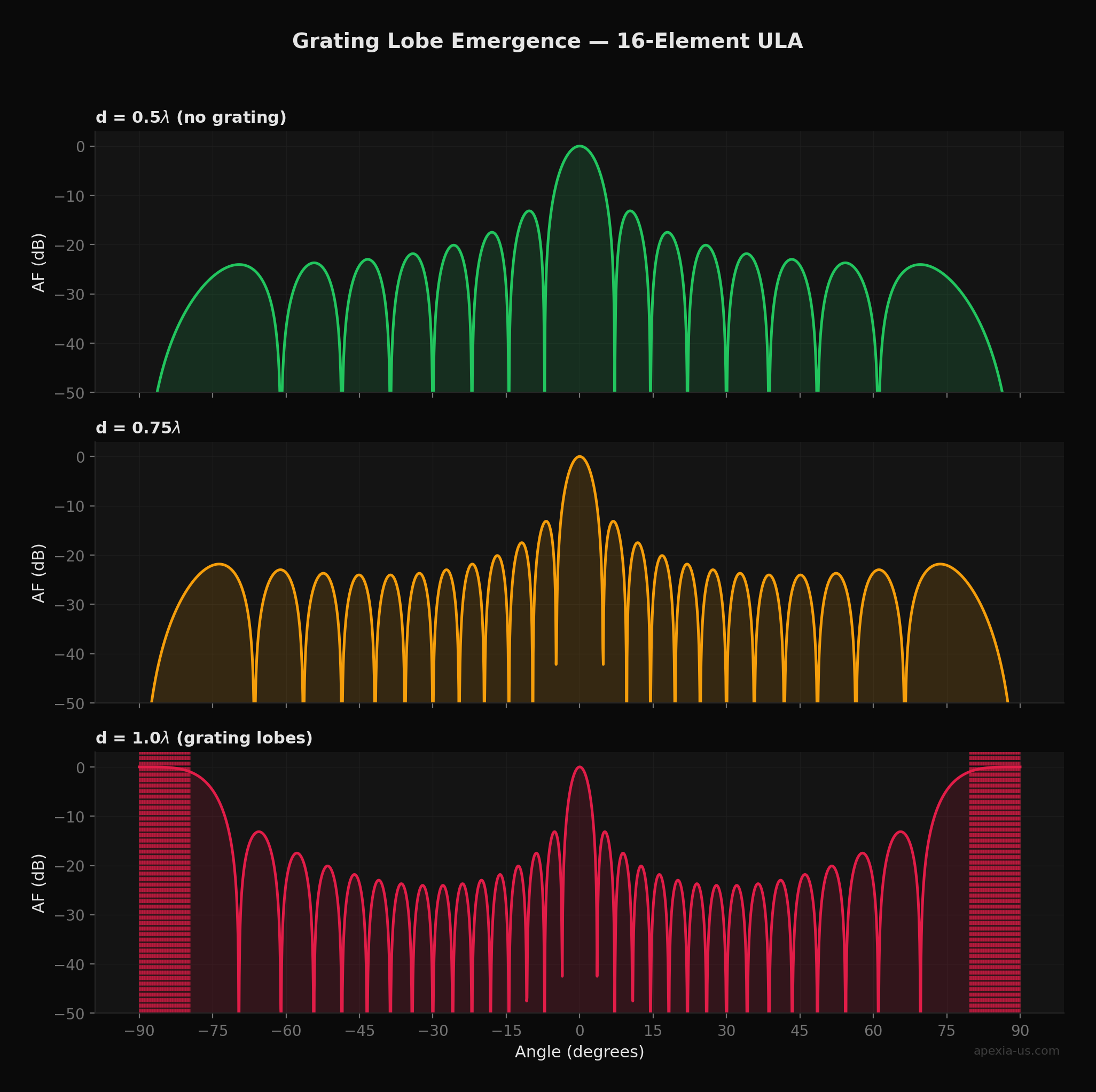
Grating lobes are full-power replicas of the main beam that appear when element spacing exceeds λ/2. They are not suppressed by amplitude tapering — they are a fundamental aliasing artifact of the spatial sampling. A grating lobe in a radar system means energy radiating (or being received from) a completely unintended direction, which is catastrophic for target detection.
Critical Design Constraint
For a phased array that must scan to ±θmax without grating lobes, element spacing must satisfy: d/λ ≤ 1/(1 + |sin θmax|). For full hemisphere scanning (±90°), this reduces to d ≤ λ/2. This is why half-wavelength spacing is the universal default for wide-scan arrays.
The simulation below makes this viscerally clear. At d = 0.5λ, the pattern is clean with a single main beam. At d = 0.75λ, strong sidelobes begin emerging at the edges of visible space. At d = 1.0λ, full grating lobes appear at ±90° — as strong as the main beam.
Planar Arrays: Extending to Two Dimensions
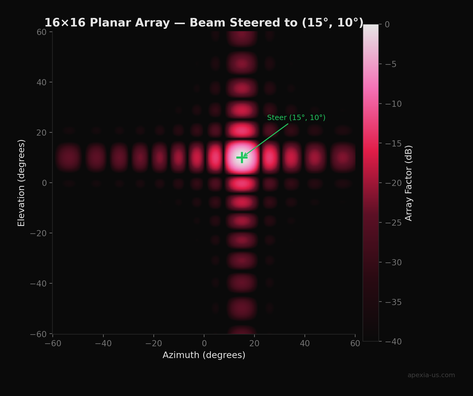
Real AESA radars use 2D planar arrays — rectangular or circular grids of elements that can steer in both azimuth and elevation simultaneously. The 2D array factor is separable for rectangular grids: AF(θx, θy) = AFx(θx) · AFy(θy), making the beamforming computation tractable even for large arrays.
The heatmap below shows the 2D beam pattern of a 16×16 planar array (256 total elements) steered to 15° azimuth and 10° elevation. The main beam is clearly visible as the bright hotspot, with the cross-shaped sidelobe structure characteristic of rectangular arrays.
FPGA Resource Scaling
A 16×16 array requires 256 complex weight multiplications per snapshot — easily parallelized across DSP slices. Modern RFSoC devices like the ZU49DR have 2,928 DSP48E2 slices, enough to implement the full beamformer for a 256-element array with room for pulse compression, Doppler processing, and CFAR detection in a single device.
FPGA Beamformer Architecture
Translating these simulations into real-time hardware is where FPGAs shine. A typical digital beamformer pipeline on an RFSoC looks like this:
- ADC Capture — Each element's RF signal is digitized by the on-chip ADC at multi-GSPS rates. The RFSoC's integrated data converters eliminate the PCB routing bottleneck.
- Digital Down-Conversion (DDC) — NCO-driven complex mixing followed by CIC/FIR decimation brings each channel to baseband at a manageable sample rate.
- Complex Weight Application — Each channel's I/Q stream is multiplied by its beamforming weight (amplitude × phase). Weights are updated from a look-up table indexed by the current beam direction.
- Coherent Summation — All weighted channels are summed to form the beam output. For multiple simultaneous beams, this stage is replicated with different weight sets.
- Post-Processing — Pulse compression (matched filter), Doppler FFT, and CFAR detection operate on the beamformed output.
The entire pipeline runs at wire speed with deterministic latency — typically under 10 µs from ADC sample to beamformed output. This is fundamentally impossible with GPU-based beamformers that must batch data, transfer to VRAM, and dispatch compute kernels. Our FPGA development services build exactly these kinds of real-time processing chains.
When to Use Each Beamforming Approach
Digital Beamforming (FPGA)
- •Full array weight control per element
- •Multiple simultaneous beams
- •Adaptive nulling and interference cancellation
- •Requires ADC per element — highest cost but maximum flexibility
Analog Beamforming
- •Phase shifters at each element, single RF combiner
- •Lower power and cost for single-beam systems
- •Limited to one beam direction at a time
- •Common in 5G mmWave and satcom terminals
Hybrid Beamforming
- •Analog subarrays with digital combining
- •Balances cost, power, and flexibility
- •Multiple beams with reduced ADC count
- •Dominant architecture in next-gen AESA radars
Key Takeaways
- 1The array factor is the product of element geometry and phase — doubling element count halves beamwidth and doubles angular resolution
- 2Electronic beam steering applies a linear phase gradient across elements, enabling microsecond scan rates with no moving parts — but beams broaden at large scan angles
- 3Amplitude tapering (Taylor, Chebyshev) suppresses sidelobes by 25-40 dB at the cost of modestly wider beams — essential for radar operation in clutter
- 4Element spacing must stay at or below λ/2 for wide-scan arrays to avoid grating lobes — a hard physical constraint that drives array geometry
- 5FPGA-based digital beamformers deliver deterministic sub-10µs latency for the entire processing chain, from ADC capture through beamformed output
Building a phased array system?
Apexia designs FPGA-based digital beamformers for AESA radar, electronic warfare, and communications systems. From array factor simulation through production RTL, we deliver real-time processing on Xilinx RFSoC platforms.